Machine Learning Part 6: Evaluating Machine Learning Models

Please Subscribe Youtube| Like Facebook | Follow Twitter

Evaluating Machine Learning Models

Evaluating machine learning models is crucial to understanding their performance and making informed decisions. In this article, we will explore essential techniques and concepts for evaluating models, including train-test split, cross-validation, performance metrics for classification and regression, and the challenges of overfitting and underfitting.

Train-test split & Cross-Validation

Train-test split

Train-test split is a technique used to evaluate the performance of machine learning models. It involves dividing the available data into two separate sets: the training set and the testing set. The training set is used to train the model, while the testing set is used to evaluate its performance on unseen data. This approach helps to estimate how well the model generalizes to new data.

import numpy as np
from sklearn.model_selection import train_test_split

# Assuming 'X' is a 2D array of input features and 'y' is a 1D array of target values
X = np.array([[1, 2], [3, 4], [5, 6]])
y = np.array([0, 1, 0])

# Splitting the data into training and testing sets
X_train, X_test, y_train, y_test = train_test_split(X, y, test_size=0.2, random_state=42)

# Printing the split data
print("X_train:")
print(X_train)
print("X_test:")
print(X_test)
print("y_train:")
print(y_train)
print("y_test:")
print(y_test)

Output

X_train:
[[3 4]
 [5 6]]
X_test:
[[1 2]]
y_train:
[1 0]
y_test:
[0]

In this example, the data has been split into a training set (X_train and y_train) and a testing set (X_test and y_test). The training set contains 80% of the data, while the testing set contains 20% of the data. The random_state parameter is set to 42 to ensure reproducibility.

Code Explanation

The code splits a dataset into training and testing sets using the train_test_split function from scikit-learn. The following steps are executed:

Step 1: Importing the necessary libraries

The numpy library is imported as np for numerical operations.
The train_test_split function is imported from the sklearn.model_selection module.

Step 2: Assuming ‘X’ is a 2D array of input features and ‘y’ is a 1D array of target values

The ‘X’ array is created as a 2D numpy array with shape (3, 2), containing input features.
The ‘y’ array is created as a 1D numpy array with shape (3,), containing target values.

Step 3: Splitting the data into training and testing sets

The train_test_split function is called to split the data into training and testing sets.
The ‘X’ and ‘y’ arrays are passed as the first two arguments.
The test_size parameter is set to 0.2, indicating that 20% of the data will be used for testing.
The random_state parameter is set to 42 for reproducibility.
The train_test_split function returns four arrays: X_train, X_test, y_train, and y_test.

Step 4: Printing the split data

The split data is printed to the console using the print function.
The X_train array, X_test array, y_train array, and y_test array are printed separately.

Cross-Validation

Cross-validation is a technique used to assess the performance of machine learning models by splitting the data into multiple subsets or “folds.” The model is trained and evaluated multiple times, with each fold serving as a testing set while the remaining folds act as the training set. This approach provides a more robust estimate of the model’s performance and helps to detect potential issues such as overfitting.

import numpy as np
from sklearn.model_selection import cross_val_score
from sklearn.linear_model import LinearRegression

# Generating a random dataset with 15 samples and 3 features
np.random.seed(42)
X = np.random.rand(15, 3)
y = np.random.rand(15)

# Creating a linear regression model
model = LinearRegression()

# Performing 5-fold cross-validation
cross_val_scores = cross_val_score(model, X, y, cv=5)

# Calculating the mean cross-validation score
mean_cv_score = cross_val_scores.mean()

# Printing the cross-validation scores and mean score
print("Cross-Validation Scores:", cross_val_scores)
print("Mean Cross-Validation Score:", mean_cv_score)

Output

Cross-Validation Scores: [ -1.67939882  -0.61181388 -28.49110176  -0.44438311 -28.40919395]
Mean Cross-Validation Score: -11.927178302902616

In this example, a random dataset is generated using the np.random.rand function. The dataset contains 15 samples and 3 features. The code creates a linear regression model and performs 5-fold cross-validation. The resulting cross-validation scores and mean score are printed.

Code Explanation

The code performs cross-validation on a linear regression model using a random dataset. The following steps are executed:

Step 1: Importing the necessary libraries

The numpy library is imported as np for numerical operations.
The cross_val_score function and LinearRegression class are imported from the sklearn.model_selection and sklearn.linear_model modules, respectively.

Step 2: Generating a random dataset

A random dataset is generated using the np.random functions.
The np.random.seed(42) statement sets a random seed for reproducibility.
The X array is created with 15 samples and 3 features, containing random numbers between 0 and 1.
The y array is created with 15 random target values.

Step 3: Creating a linear regression model

A linear regression model is created using the LinearRegression class.
An instance of the LinearRegression class is created as model.

Step 4: Performing 5-fold cross-validation

Cross-validation is performed using the cross_val_score function.
The cross_val_score function is called with the model, X, y, and cv=5 as arguments.
The cv parameter specifies 5-fold cross-validation.
The cross-validation scores for each fold are assigned to the cross_val_scores variable.

Step 5: Calculating the mean cross-validation score

The mean cross-validation score is calculated by taking the mean of the cross_val_scores.
The mean method is called on the cross_val_scores to calculate the mean.
The mean cross-validation score is assigned to the mean_cv_score variable.

Step 6: Printing the cross-validation scores and mean score

The cross-validation scores and mean cross-validation score are printed to the console using the print function.

Performance Metrics for Classification and Regression

Performance metrics are used to measure the effectiveness of machine learning models in classification and regression tasks.

Performance Metrics for Classification

For classification tasks, common performance metrics include:

Accuracy: The proportion of correct predictions to the total number of predictions.
Precision: The ability of the model to correctly identify positive instances.
Recall: The ability of the model to correctly identify all positive instances.
F1-score: The harmonic mean of precision and recall, providing a balanced measure of performance.

from sklearn.metrics import accuracy_score, precision_score, recall_score, f1_score

# Example values for y_true and y_pred
y_true = [0, 1, 1, 0, 1]
y_pred = [0, 1, 0, 0, 1]

# Calculating classification performance metrics
accuracy = accuracy_score(y_true, y_pred)
precision = precision_score(y_true, y_pred)
recall = recall_score(y_true, y_pred)
f1 = f1_score(y_true, y_pred)

# Output the results
print("Accuracy:", accuracy)
print("Precision:", precision)
print("Recall:", recall)
print("F1 Score:", f1)

Output

Accuracy: 0.8
Precision: 1.0
Recall: 0.6666666666666666
F1 Score: 0.8

Code Explanation

The code calculates classification performance metrics, including accuracy, precision, recall, and F1 score, based on the true and predicted labels. The following steps are executed:

Step 1: Importing the necessary libraries

The accuracy_score, precision_score, recall_score, and f1_score functions are imported from the sklearn.metrics module.

Step 2: Example values for y_true and y_pred

The y_true list is created as [0, 1, 1, 0, 1], representing the true labels.
The y_pred list is created as [0, 1, 0, 0, 1], representing the predicted labels.

Step 3: Calculating classification performance metrics

The classification performance metrics are calculated using the appropriate functions.
The accuracy_score function is called with y_true and y_pred as arguments to calculate the accuracy.
The precision_score function is called with y_true and y_pred as arguments to calculate the precision.
The recall_score function is called with y_true and y_pred as arguments to calculate the recall.
The f1_score function is called with y_true and y_pred as arguments to calculate the F1 score.

Step 4: Output the results

The calculated classification performance metrics are printed to the console using the print function.
The accuracy, precision, recall, and F1 score are printed separately.

Performance Metrics for Regression

For regression tasks, common performance metrics include:

Mean Squared Error (MSE): The average of the squared differences between the predicted and actual values.
Mean Absolute Error (MAE): The average of the absolute differences between the predicted and actual values.
R-squared (R2): The proportion of the variance in the dependent variable explained by the model.

from sklearn.metrics import mean_squared_error, mean_absolute_error, r2_score

# Example values for y_true and y_pred
y_true = [1.2, 2.4, 3.6, 4.8]
y_pred = [1.0, 2.0, 3.5, 5.0]

# Calculating regression performance metrics
mse = mean_squared_error(y_true, y_pred)
mae = mean_absolute_error(y_true, y_pred)
r2 = r2_score(y_true, y_pred)

# Output the results
print("Mean Squared Error (MSE):", mse)
print("Mean Absolute Error (MAE):", mae)
print("R^2 Score:", r2)

Output

Mean Squared Error (MSE): 0.06249999999999999
Mean Absolute Error (MAE): 0.22500000000000003
R^2 Score: 0.9652777777777778

Code Explanation

The code calculates regression performance metrics, including mean squared error (MSE), mean absolute error (MAE), and R-squared score, based on the true and predicted values. The following steps are executed:

Step 1: Importing the necessary libraries

The mean_squared_error, mean_absolute_error, and r2_score functions are imported from the sklearn.metrics module.

Step 2: Example values for y_true and y_pred

The y_true list is created as [1.2, 2.4, 3.6, 4.8], representing the true values.
The y_pred list is created as [1.0, 2.0, 3.5, 5.0], representing the predicted values.

Step 3: Calculating regression performance metrics

The regression performance metrics are calculated using the appropriate functions.
The mean_squared_error function is called with y_true and y_pred as arguments to calculate the MSE.
The mean_absolute_error function is called with y_true and y_pred as arguments to calculate the MAE.
The r2_score function is called with y_true and y_pred as arguments to calculate the R-squared score.

Step 4: Output the results

The calculated regression performance metrics are printed to the console using the print function.
The MSE, MAE, and R-squared score are printed separately.

Overfitting and Underfitting

Overfitting occurs when a machine learning model performs exceptionally well on the training data but fails to generalize to new, unseen data. This typically happens when the model becomes too complex and learns the noise and idiosyncrasies of the training set. On the other hand, underfitting occurs when the model is too simple to capture the underlying patterns in the data and performs poorly on both the training and testing sets.

Both overfitting and underfitting can be addressed by using appropriate evaluation techniques, such as cross-validation, and by selecting models with the right level of complexity or through regularization techniques.

Below code provides demonstration of overfitting and underfitting by comparing learning curves for different model complexities. It helps illustrate how the training and testing errors vary with the degree of polynomial regression.

By observing the learning curves, you can get a better understanding of the trade-off between model complexity and generalization performance. It allows you to identify scenarios of overfitting (high training error, large gap with testing error) and underfitting (high training and testing errors without a clear gap).

import numpy as np
import matplotlib.pyplot as plt
from sklearn.model_selection import learning_curve
from sklearn.svm import SVR
from sklearn.preprocessing import PolynomialFeatures
from sklearn.pipeline import make_pipeline

# Example data for demonstration purposes
X = np.array([[1], [2], [3], [4], [5]])  # Input features
y = np.array([2, 4, 6, 8, 10])  # Target variable

# Define different degrees of polynomial regression models
degrees = [1, 3, 5, 9]

# Plotting the learning curves for different model complexities
plt.figure(figsize=(10, 6))

for degree in degrees:
    # Create a polynomial regression model
    model = make_pipeline(PolynomialFeatures(degree), SVR())

    # Calculate the learning curve
    train_sizes, train_scores, test_scores = learning_curve(
        model, X, y, cv=5, scoring='neg_mean_squared_error', train_sizes=np.linspace(0.1, 1.0, 10))

    # Calculate the mean training and testing errors
    mean_train_errors = -np.mean(train_scores, axis=1)
    mean_test_errors = -np.mean(test_scores, axis=1)

    # Plot the learning curve
    plt.plot(train_sizes, mean_train_errors, label=f'Training Error (Degree {degree})')
    plt.plot(train_sizes, mean_test_errors, label=f'Testing Error (Degree {degree})')

plt.xlabel('Number of Training Examples')
plt.ylabel('Mean Squared Error')
plt.title('Learning Curves for Polynomial Regression')
plt.legend()
plt.show()

Output

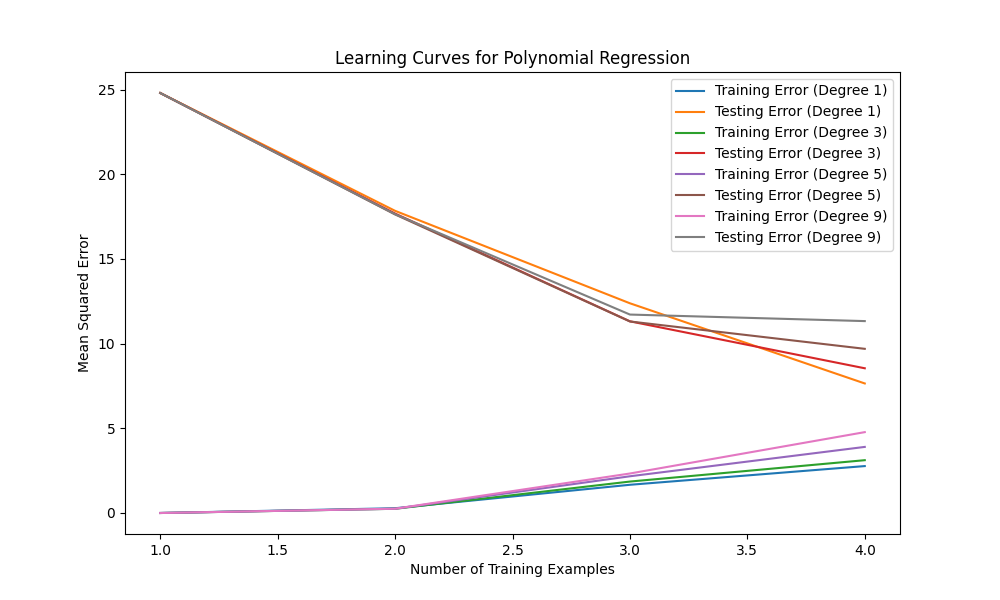
In this code, we introduce different degrees of polynomial regression models by using PolynomialFeatures from scikit-learn. We create polynomial regression models with degrees 1, 3, 5, and 9. The learning curves for these models are then plotted, showing the mean squared errors for both training and testing sets.

By observing the learning curves, you can identify the following scenarios:

Overfitting: If the training error is significantly lower than the testing error and there is a large gap between the two curves, it suggests overfitting. This is the case when the degree is high (e.g., degree 9). The model is too complex and fits the noise in the training data, resulting in poor generalization.

Underfitting: If both the training error and testing error are high, and there is no clear gap between the two curves, it indicates underfitting. This is the case when the degree is low (e.g., degree 1). The model is too simple to capture the underlying patterns in the data.

Good fit: A good fit is achieved when the training and testing errors are both low and relatively close to each other. This can be observed for an intermediate degree (e.g., degree 3 or 5).

Please note that this example uses polynomial regression as a demonstration. In real-world scenarios, you may encounter overfitting and underfitting with different types of models and different datasets. It’s important to select an appropriate model complexity that balances the bias-variance tradeoff and generalizes well to unseen data.

Code Explanation

The code generates learning curves for polynomial regression models of different degrees using example data. The following steps are executed:

Step 1: Importing the necessary libraries

The numpy library is imported as np for numerical operations.
The matplotlib.pyplot library is imported as plt for data visualization.
The learning_curve, SVR, PolynomialFeatures, and make_pipeline functions are imported from the sklearn.model_selection, sklearn.svm, sklearn.preprocessing, and sklearn.pipeline modules, respectively.

Step 2: Example data for demonstration purposes

The X array is created as a 2D numpy array with shape (5, 1), containing input features.
The y array is created as a 1D numpy array with shape (5,), containing target variable values.

Step 3: Define different degrees of polynomial regression models

The degrees variable is defined as a list of different polynomial degrees. In this example, it is set to [1, 3, 5, 9].

Step 4: Plotting the learning curves for different model complexities

A new figure is created using the plt.figure(figsize=(10, 6)) function.

Step 5: Looping over different degrees

A for loop is used to iterate over each degree in the degrees list.

Step 6: Create a polynomial regression model

Inside the loop, a polynomial regression model is created using the make_pipeline function.
The PolynomialFeatures(degree) transformer is used to generate polynomial features.
The SVR model is used as the regressor in the pipeline.
The model is assigned to the variable model.

Step 7: Calculate the learning curve

The learning_curve function is called to calculate the learning curve for the current model.
The learning_curve function is called with the model, X, y, cv=5, scoring=’neg_mean_squared_error’, and train_sizes=np.linspace(0.1, 1.0, 10) as arguments.
The cv parameter specifies 5-fold cross-validation.
The scoring parameter is set to ‘neg_mean_squared_error’ to use mean squared error as the evaluation metric.
The train_sizes parameter is set to np.linspace(0.1, 1.0, 10) to define different training set sizes.

Step 8: Calculate the mean training and testing errors

The mean training and testing errors are calculated by taking the negative mean of the train_scores and test_scores arrays along axis=1, respectively.
The -np.mean function is applied to the train_scores and test_scores arrays to calculate the mean values.
The mean training errors are assigned to the mean_train_errors variable.
The mean testing errors are assigned to the mean_test_errors variable.

Step 9: Plot the learning curve

The learning curve is plotted using the plt.plot() function inside the loop.
The mean_train_errors and mean_test_errors are plotted against train_sizes.
The label for the training error curve is set to ‘Training Error (Degree {degree})’, where {degree} represents the current degree in the loop.
The label for the testing error curve is set to ‘Testing Error (Degree {degree})’.
The x-axis label is set to ‘Number of Training Examples’ using the plt.xlabel() function.
The y-axis label is set to ‘Mean Squared Error’ using the plt.ylabel() function.
The title of the plot is set to ‘Learning Curves for Polynomial Regression’ using the plt.title() function.
A legend is added to the plot using the plt.legend() function.
The plot is displayed using the plt.show() function.

Conclusion

Evaluating machine learning models involves a combination of techniques such as train-test split, cross-validation, and performance metrics for classification and regression. By understanding these concepts and addressing challenges like overfitting and underfitting, we can effectively assess the performance of machine learning models and make informed decisions in real-world applications.

Machine Learning In Python Beginner Tutorial Series

Please Subscribe Youtube| Like Facebook | Follow Twitter

Machine Learning Part 6: Evaluating Machine Learning Models

Evaluating Machine Learning Models

Train-test split & Cross-Validation

Train-test split

Output

Code Explanation

Cross-Validation

Output

Code Explanation

Performance Metrics for Classification and Regression

Performance Metrics for Classification

Output

Code Explanation

Performance Metrics for Regression

Output

Code Explanation

Overfitting and Underfitting

Output

Code Explanation

Conclusion

Published by ProgramTown

Leave a Reply Cancel reply