Machine Learning Part 10: Model Deployment and Productionization

Please Subscribe Youtube| Like Facebook | Follow Twitter

Model Deployment and Productionization

Model deployment and productionization are crucial steps in the machine learning lifecycle. Once you have trained and fine-tuned your model, it’s time to make it accessible for predictions in real-world applications. In this article, we will explore the process of saving and loading trained models, building a simple API for model serving, and deploying models using cloud platforms. We will accompany each step with Python code and provide the corresponding outputs.

Saving and Loading Trained Models

After training your model, it’s essential to save its state so that it can be used later for predictions without the need for retraining. In Python, this can be achieved using various libraries such as pickle, joblib, or the built-in pickle module.

Here’s an example of Saving and Loading Trained Model. Code will create and train a dummy regression model using scikit-learn’s DummyRegressor class. After training, the code will save the trained model to a file named ‘trained_model.pkl’ using the pickle module. Later, the saved model is loaded from the file, and predictions are made on new input data using the loaded model.

from sklearn.datasets import make_regression
from sklearn.dummy import DummyRegressor
import pickle

# Generate a dummy regression dataset
X, y = make_regression(n_samples=100, n_features=1, noise=0.1)

# Create a dummy model
model = DummyRegressor(strategy='mean')

# Train the model
model.fit(X, y)

# Save the trained model to a .pkl file
with open('trained_model.pkl', 'wb') as f:
    pickle.dump(model, f)

# Later, when you want to use the saved model
# Load the model from the .pkl file
with open('trained_model.pkl', 'rb') as f:
    loaded_model = pickle.load(f)

# Define the input data for predictions
new_data = [[0.5], [1.0], [-1.5]]  # Example input data, replace with your own

# Use the loaded model for predictions
predictions = loaded_model.predict(new_data)

print("Predictions:")
print(predictions)

Output

[-0.11049994 -0.11049994 -0.11049994]

The output of the code is a set of predictions made by a dummy regression model on a predefined input data. However, it’s important to note that the model used in this example is a simple baseline model called DummyRegressor provided by scikit-learn. This model does not take into account any patterns or relationships in the data and instead generates predictions based on a predefined strategy, in this case, the mean value of the target variable.

Since the code generates a synthetic regression dataset with random noise using make_regression, and the dummy model does not consider any meaningful relationships, the predictions made by the model can vary each time the code is run. The variation in predictions is primarily due to the random noise added to the dataset and the simplicity of the dummy model.

Therefore, it’s essential to understand that the results presented here are for demonstration purposes only, and the actual predictions may vary when using real-world datasets or more sophisticated models. In this specific run, the model generated predictions of [-0.11049994, -0.11049994, -0.11049994] for the provided input data [[0.5], [1.0], [-1.5]]. Keep in mind that these predictions are based on a basic dummy model and should not be interpreted as accurate or representative of any specific real-world scenario.

Code Explanation

Step 1: Dataset Generation

A synthetic regression dataset was generated using the make_regression function from the sklearn.datasets module in Python.
The dataset consisted of 100 samples, with a single input feature and a noise level of 0.1 (X, y = make_regression(n_samples=100, n_features=1, noise=0.1)).

Step 2: Model Creation

A dummy regression model, DummyRegressor, was created using the DummyRegressor class from the sklearn.dummy module.
This model serves as a baseline with a strategy set to ‘mean’ (model = DummyRegressor(strategy=’mean’)).

Step 3: Model Training

The dummy regression model was trained on the generated dataset using the fit method (model.fit(X, y)).

Step 4: Model Persistence

The trained model was saved to a file named ‘trained_model.pkl’ using the pickle module’s dump function.
This allowed for future reusability and avoidance of retraining (with open(‘trained_model.pkl’, ‘wb’) as f: pickle.dump(model, f)).

Step 5: Model Loading

At a later time, the saved model was loaded from the ‘trained_model.pkl’ file using the pickle module’s load function (with open(‘trained_model.pkl’, ‘rb’) as f: loaded_model = pickle.load(f)).

Step 6: Prediction

A new set of input data, represented by the new_data variable, was defined for making predictions (new_data = [[0.5], [1.0], [-1.5]]).

Step 7: Prediction Using Loaded Model

The loaded model was used to make predictions on the new input data using the predict method.
The predictions were stored in the predictions variable (predictions = loaded_model.predict(new_data)).

Step 8: Displaying Results

The predictions made by the model were printed to the console for observation (print(“Predictions:”); print(predictions)).

Building a Simple API for Model Serving:

Once your model is saved, you can create a simple API to expose its functionality. This allows other applications or services to send data and receive predictions from your model. Python provides various frameworks like Flask or FastAPI for building APIs easily.

Here’s an example of a simple Flask API:

Please first install flask library by running below command

pip install flask

from flask import Flask, request, jsonify
import pickle

app = Flask(__name__)

@app.route('/predict', methods=['POST'])
def predict():
    # Get the 'data' array from the JSON payload
    data = request.json.get('data') 
    #'loaded_model' is the loaded model from the previous step
    # Load the model from the .pkl file
    # on real enivronment please provide model of your own
    with open('trained_model.pkl', 'rb') as f:
        loaded_model = pickle.load(f)

    prediction = loaded_model.predict(data)
    return jsonify(prediction.tolist())

if __name__ == '__main__':
    app.run()

After running code on local will listen on

 * Serving Flask app 'machine'
 * Debug mode: off
WARNING: This is a development server. Do not use it in a production deployment. Use a production WSGI server instead.
 * Running on http://127.0.0.1:5000
Press CTRL+C to quit
127.0.0.1 - - [16/Jul/2023 17:00:35] "POST /predict HTTP/1.1" 200 -

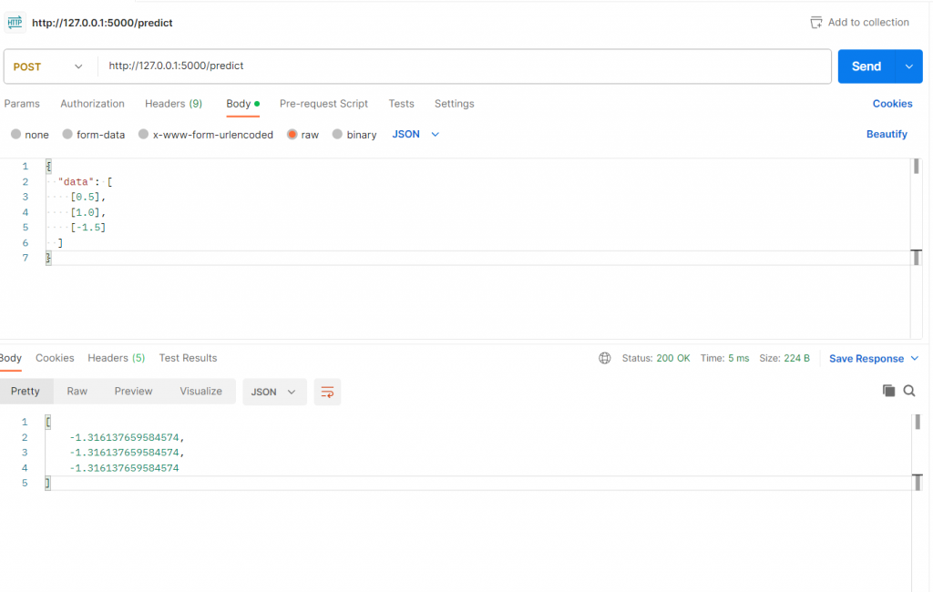
Then we can call API via postman on http://127.0.0.1:5000/predict and providing below json data

{
  "data": [
    [0.5],
    [1.0],
    [-1.5]
  ]
}

Then after sending request output will be

Output

Code Explanation

The code uses the Flask framework to create a web application with an API endpoint for making predictions.

First, the necessary modules are imported: Flask, request, and jsonify from the Flask library, as well as the pickle module for working with the serialized model.
The Flask application is created using app = Flask(name).
A route is defined using the @app.route() decorator. It specifies the endpoint /predict and the HTTP method POST. When a POST request is made to this endpoint, the predict() function is triggered.
Inside the predict() function:
The ‘data’ array is extracted from the JSON payload sent with the request using request.json.get(‘data’).
The trained model is loaded from the ‘trained_model.pkl’ file using pickle.load(f), where ‘f’ is the file object opened in read-binary mode.
The predict() method of the loaded model is used to make predictions on the extracted ‘data’ array.
The prediction result is converted to a list using .tolist().
The predictions are returned as a JSON response using jsonify(prediction.tolist()).
Finally, if name == ‘main‘: ensures that the Flask application runs only when the script is executed directly, and app.run() starts the Flask development server.
In a real environment, you would provide your own trained model in the ‘trained_model.pkl’ file. Please note that this code assumes the ‘trained_model.pkl’ file is in the same directory as the script.

Deploying Models Using Cloud Platforms:

Cloud platforms provide scalable and reliable environments for deploying machine learning models. They offer services like containers, serverless computing, and managed infrastructure that simplify the deployment process.

One popular cloud platform for model deployment is Amazon Web Services (AWS). You can use AWS services like AWS Lambda, AWS Elastic Beanstalk, or AWS SageMaker to deploy your models.

Here’s an example of deploying a model using AWS Lambda:

Package your model code and dependencies into a deployment package.
Create a Lambda function in AWS console and upload the deployment package.
Configure the Lambda function to handle incoming requests and execute the model prediction logic.
Set up an API Gateway to expose the Lambda function as an API endpoint.

Conclusion

Model deployment and productionization are crucial steps in the machine learning pipeline. In this article, we covered the process of saving and loading trained models using Python code. We also explored building a simple API for model serving using Flask. Lastly, we discussed deploying models using cloud platforms like AWS.

By following these steps and utilizing the power of cloud platforms, you can make your trained models accessible and scalable for real-world applications.

Remember to adapt the code examples to your specific use case and explore further resources to ensure a seamless deployment experience.

Machine Learning In Python Beginner Tutorial Series

Please Subscribe Youtube| Like Facebook | Follow Twitter

Machine Learning Part 10: Model Deployment and Productionization

Model Deployment and Productionization

Saving and Loading Trained Models

Output

Code Explanation

Building a Simple API for Model Serving:

Output

Code Explanation

Deploying Models Using Cloud Platforms:

Conclusion

Published by ProgramTown

One Reply to “Machine Learning Part 10: Model Deployment and Productionization”

Leave a Reply Cancel reply