Machine Learning Part 5: Introduction to Unsupervised Learning Algorithms
Please Subscribe Youtube| Like Facebook | Follow Twitter
Unsupervised Learning Algorithms
This article provides an overview of three popular unsupervised learning algorithms: K-means clustering, hierarchical clustering, and Principal Component Analysis (PCA). Along with explanations, each algorithm will be accompanied by Python code and their respective outputs to demonstrate their applications.
Unsupervised Learning
Unsupervised learning is a branch of machine learning where the goal is to discover patterns, structures, and relationships within a dataset without the presence of labeled examples. Unlike supervised learning, unsupervised learning does not rely on predefined target variables or explicit feedback. Instead, it explores the inherent structure and properties of the data to extract meaningful insights.
Unsupervised Algorithms
Unsupervised algorithms are computational methods used in unsupervised learning to extract meaningful information from unlabeled data. These algorithms explore the data’s inherent structure and patterns without any explicit guidance.
In the field of machine learning, unsupervised learning algorithms play a crucial role in analyzing and understanding data without the need for labeled examples. Unsupervised learning techniques help identify patterns, structures, and relationships within datasets.
K-means Clustering
K-means clustering is a versatile algorithm used for grouping similar data points into clusters. The algorithm iteratively assigns data points to clusters by minimizing the within-cluster variance. Here’s an example of implementing K-means clustering in Python:
# Importing the required libraries
from sklearn.cluster import KMeans
import numpy as np

# Assuming you have a dataset named "data" as a numpy array
data = np.array([[1, 2], [3, 4], [5, 6], [7, 8]])

# Creating an instance of K-means clustering algorithm
kmeans = KMeans(n_clusters=3, n_init=10)

# Fitting the algorithm on the dataset
kmeans.fit(data)

# Getting the cluster labels for each data point
labels = kmeans.labels_

# Printing the cluster labels
print(labels)
Output
[0 0 2 1]
Code Explanation
The code performs K-means clustering using the scikit-learn library. The following steps are executed:
Step 1: Importing the required libraries
- The necessary libraries are imported:
- The KMeans class from the sklearn.cluster module, which provides the implementation of the K-means clustering algorithm.
- The numpy library is imported as np for numerical operations.
Step 2: Creating the dataset
- A dataset named “data” is assumed to be provided as a numpy array. It contains four data points with two features each.
Step 3: Creating an instance of the K-means algorithm
- An instance of the K-means algorithm is created with n_clusters=3, indicating that the algorithm should identify three clusters in the data.
- The n_init parameter is set to 10, specifying the number of times the algorithm will be run with different centroid seeds.
Step 4: Fitting the algorithm on the dataset
- The K-means algorithm is fitted to the dataset using the fit method.
- This calculates the cluster centroids and assigns each data point to its nearest centroid.
Step 5: Getting the cluster labels
- The labels variable is assigned the cluster labels for each data point.
- These labels indicate the cluster assignment for each data point based on the fitted K-means algorithm.
Step 6: Printing the cluster labels
- The cluster labels [0 0 2 1] are printed to the console using the print function.
Hierarchical Clustering
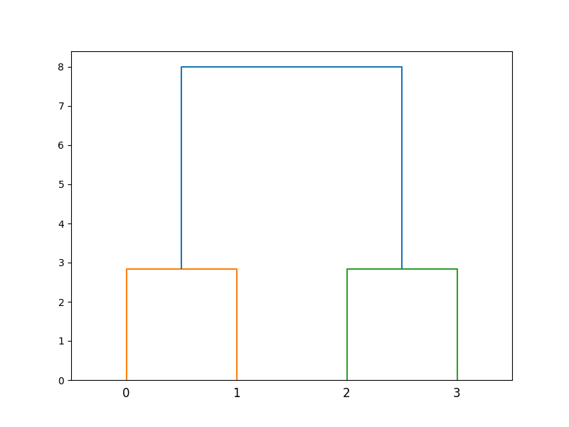
Hierarchical clustering is an algorithm that builds a hierarchy of clusters by recursively merging or splitting them based on the similarity between data points. The result is a tree-like structure called a dendrogram. Let’s see how to perform hierarchical clustering using Python:
# Importing the required libraries
from scipy.cluster.hierarchy import linkage, dendrogram
import matplotlib.pyplot as plt
import numpy as np

# Assuming you have a dataset named "data" as a numpy array
data = np.array([[1, 2], [3, 4], [5, 6], [7, 8]])

# Performing hierarchical clustering
linkage_matrix = linkage(data, method='ward')

# Plotting the dendrogram
plt.figure(figsize=(8, 6))
dendrogram(linkage_matrix)
plt.show()
Output

Code Explanation
The code performs hierarchical clustering and plots a dendrogram using the scipy and matplotlib libraries. The following steps are executed:
Step 1: Importing the required libraries
- The necessary libraries are imported:
- The linkage and dendrogram functions are imported from the scipy.cluster.hierarchy module. These functions are used for hierarchical clustering and dendrogram plotting.
- The matplotlib.pyplot module is imported as plt for creating visualizations.
- The numpy library is imported as np for numerical operations.
Step 2: Creating the dataset
- A dataset named “data” is assumed to be provided as a numpy array. It contains four data points with two features each.
Step 3: Performing hierarchical clustering
- The linkage function is used to calculate the linkage matrix for hierarchical clustering.
- The ‘ward’ method is specified to compute the distance between clusters.
Step 4: Plotting the dendrogram
- A figure with a size of 8×6 inches is created using the plt.figure function.
- The dendrogram function is then called to plot the dendrogram based on the linkage matrix.
- Finally, the plt.show function is used to display the dendrogram.
Principal Component Analysis (PCA)
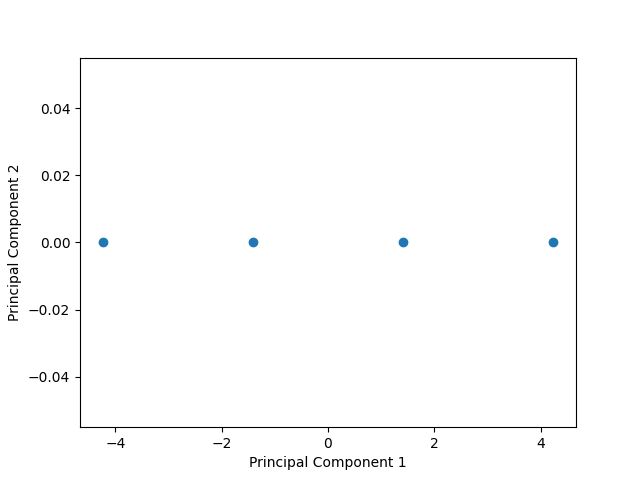
Principal Component Analysis (PCA) is a dimensionality reduction technique that transforms a high-dimensional dataset into a lower-dimensional representation while preserving its essential features. PCA identifies the principal components that capture the most significant variance in the data. Here’s an example of performing PCA in Python:
# Importing the required libraries
from sklearn.decomposition import PCA
import matplotlib.pyplot as plt
import numpy as np

# Assuming you have a dataset named "data" as a numpy array
data = np.array([[1, 2], [3, 4], [5, 6], [7, 8]])

# Creating an instance of PCA
pca = PCA(n_components=2)

# Fitting the PCA model on the dataset
pca.fit(data)

# Transforming the data to the lower-dimensional space
transformed_data = pca.transform(data)

# Plotting the transformed data
plt.scatter(transformed_data[:, 0], transformed_data[:, 1])
plt.xlabel('Principal Component 1')
plt.ylabel('Principal Component 2')
plt.show()
Output

Code Explanation
The code performs Principal Component Analysis (PCA) on a dataset using the scikit-learn and matplotlib libraries. The following steps are executed:
Step 1: Importing the required libraries
- The necessary libraries are imported:
- The PCA class is imported from the sklearn.decomposition module, which provides the implementation of PCA.
- The matplotlib.pyplot module is imported as plt for creating visualizations.
- The numpy library is imported as np for numerical operations.
Step 2: Creating the dataset
- A dataset named “data” is assumed to be provided as a numpy array. It contains four data points with two features each.
Step 3: Creating an instance of PCA
- An instance of the PCA class is created with n_components=2, indicating that the dimensionality of the data should be reduced to two principal components.
Step 4: Fitting the PCA model on the dataset
- The fit method is called on the PCA instance to fit the PCA model on the dataset.
Step 5: Transforming the data to the lower-dimensional space
- The transform method is used to transform the original data to the lower-dimensional space defined by the principal components.
Step 6: Plotting the transformed data
- The scatter plot is created using the plt.scatter function.
- The transformed data is plotted, with the first principal component on the x-axis and the second principal component on the y-axis.
- The plt.xlabel and plt.ylabel functions are used to label the axes. Finally, the plt.show function is called to display the plot.
Conclusion
Unsupervised learning algorithms, such as K-means clustering, hierarchical clustering, and Principal Component Analysis (PCA), offer powerful tools for exploring and analyzing datasets without the need for labeled data. Python provides a rich ecosystem of libraries, making it easy to implement and visualize these algorithms. By leveraging these techniques, data scientists can gain valuable insights into the underlying structures and patterns within their data.
Machine Learning In Python Beginner Tutorial Series
- Machine Learning Part 1: Introduction
- Machine Learning Part 2: Understanding Data Preprocessing For Machine Learning
- Machine Learning Part 3: Exploratory Data Analysis for Machine Learning
- Machine Learning Part 4: Introduction to Supervised Learning Algorithms
- Machine Learning Part 5: Introduction to Unsupervised Learning Algorithms
- Machine Learning Part 6: Evaluating Machine Learning Models
- Machine Learning Part 7: Deep Learning and Neural Networks
- Machine Learning Part 8: Natural Language Processing (NLP)
- Machine Learning Part 9: Recommender Systems
- Machine Learning Part 10: Model Deployment and Productionization
 Mens Winter Single Breasted Big Pockets Mid Long Casual Coats
 Mens Contrast Patchwork Flap Pocket Decoration Short Sleeve T-Shirts
 Orange Pi 800 Development Board 4GB RAM 64GB
 Mens Casual Corduroy Hooded Button Pocket Comfy Shirts
 E500 1.83 inch HD Screen ECG Monitor Heart Rate Blood Pressure
 35L Outdoor Backpack Men Women Waterproof Travel Trekking Backpack
 Home Steam Sauna Box Steam Room Fumigation Machine Steam Sauna Bath Sauna Heater
 GPD WIN Max 2 LPDDR5 32GB RAM 2TB SSD AMD R7 6800U Windows 11 Gaming Notebook 10.1 Inch Laptop Portable Game Computer Handheld Game Console US Plug
 SKYLOONG GK64X GK64XS Keyboard Kit RGB Hot Swappable 60% Programmable bluetooth Wired Case Customized Kit PCB Mounting Plate Case with Replacable Space Key